Quantcast
Channel: CDH – Cloudera Engineering Blog
Viewing all 426 articles
Browse latest View live

CDH6.2 – Cloudera Search Attribute Based Access Control Part 1

$
0
0

Cloudera Search is a highly scalable and flexible search solution based on Apache Solr which enables exploration, discovery and analytics over massive, unstructured and semi-structured datasets (for example logs, emails, dna-strings, claims forms, jpegs, xls sheets, etc). It has been adopted by a large number of Cloudera customers across a wide range of industries for high ROI and SLA-bound workloads, with many of those having strict requirements around security and compliance.

In CDH 5.1.0 we introduced document-level security for Cloudera Search using Apache Sentry. This model provided a mechanism where user groups could be assigned one or more roles which would then be matched against tokens specified within a Solr document. This simple mechanism meant that it was possible to essentially tag documents in order to control access to them.

As an example, in order to provide a Purpose Based Access Control (PBAC) model in compliance with GDPR Article 6, a document may be tagged according to the purposes that the subject has consented, for example [“marketing“, “product-development“] and this would mean that only users who have either the “marketing” or “product-development” roles (or both) could see the document.

In CDH6.2 we introduce two new features to Cloudera Search relating to document-level security. The first extends this role-based model by adding a conjunctive match capability and the second introduces attribute-based access control to protect documents based on multiple fields and against user attributes retrieved from an attribute store.

In this blog we will explore the conjunctive match capability, and part 2 will explore the attribute-based access control feature.

Conjunctive Match

The CDH5.1 role-based model provided a disjunctive, or OR based predicate – where the user must have token1 or token2 or token3 etc. With conjunctive match we simply ensure that all of the tokens applied to a document must be assigned to the user in order for access to be granted. This is sometimes known as AND based predicates, or AND groups.

This might be used in scenarios where information is limited to extreme intersections of users, for example in Mergers and Acquisitions where you might need to have information that cannot be seen by both parties:

{
id: "document1",
sentry_auth: ["cldr", "mergerteam"],
sentry_auth_count: 2,
text: "Some text that can only be seen by some of the merger team"
}
{
id: "document2",
sentry_auth: ["hdp", "mergerteam"],
sentry_auth_count: 2,
text: "Some text that can only be seen by different members of the merger team"
}
{
id: "document3",
sentry_auth: ["mergerteam"],
sentry_auth_count: 1,
text: "All members of the merger team can see this"
}

As with the existing document-level security in Cloudera Search we control this using the solrconfig.xml file, and then map users to roles using Apache Sentry:

<queryParser name="subset" class="org.apache.solr.handler.component.SubsetQueryPlugin" />
<searchComponent name="queryDocAuthorization" class="org.apache.solr.handler.component.QueryDocAuthorizationComponent">
  <bool name="enabled">true</bool>
<str name="matchMode">CONJUNCTIVE</str>
<str name="sentryAuthField">sentry_auth</str>
<str name="tokenCountField">sentry_auth_count</str>
  <str name="allRolesToken">anybody</str>
  <str name="allow_missing_val">true</str>
  <str name="qParser">subset</str>
</searchComponent>

To make the conjunctive match capability work, we’re introducing three new things:

  1. A matchMode attribute, which we set to CONJUNCTIVE
  2. A tokenCountField which needs to specify the minimum number of values that the user needs to match on a per-document basis
  3. We define the Subset query, which in this instance we’ve called “subset”, which is the default name.

The allRolesToken is a field which is implicitly given to all users (for example as a default role), and similarly the allow_missing_val capabilities defines whether permission should be granted to documents who do not have a value for the sentryAuthField.

Running a query against this collection with the debug attribute set shows us the actual filter that is being appended onto the query as a predicate:

CDH 6.2 Cloudera Search

Using the debug attribute, it can sometimes be slightly easier to understand why specific documents are or are not being filtered.

Conclusion

This blog introduces the conjunctive match feature delivered for Cloudera Search in CDH6.2. Part 2 will explore the attribute-based access control feature.


Acknowledgements
SENTRY-2482 was delivered by a multi-functional team, including Hrishikesh Gadre, David Beech, Zsolt Gyulavari, Kalyan Kumar Kalvagadda, Tristan Stevens and Eva Nahari.

Tristan Stevens is a Principal Solutions Architect at Cloudera

The post CDH6.2 – Cloudera Search Attribute Based Access Control Part 1 appeared first on Cloudera Engineering Blog.


CDH6.2 – Cloudera Search Attribute Based Access Control Part 2

$
0
0

Cloudera Search is a highly scalable and flexible search solution based on Apache Solr which enables exploration, discovery and analytics over massive, unstructured and semi-structured datasets (for example logs, emails, dna-strings, claims forms, jpegs, xls sheets, etc). It has been adopted by a large number of Cloudera customers across a wide range of industries for high ROI and SLA-bound workloads, with many of those having strict requirements around security and compliance.

In CDH6.2 we introduce two new features to Cloudera Search relating to document-level security. The first extends this role-based model by adding a conjunctive match capability and the second introduces attribute-based access control to protect documents based on multiple fields and against user attributes retrieved from an attribute store.

Part 1 explored the conjunctive match capability, and this part will explore the attribute-based access control feature.

Attribute Based Access Control

Attribute Based Access Control is defined by NIST as “An access control method where subject requests to perform operations on objects are granted or denied based on assigned attributes of the subject, assigned attributes of the object, environment conditions, and a set of policies that are specified in terms of those attributes and conditions.”

In this model, we are defining a set of policies in the solrconfig.xml file where we are going to construct a set of predicates based on a user’s attributes, which will then be applied to enforce access control against a number of fields defined on each document. Cloudera’s reference architecture is illustrated in Figure 1. It differs from the NIST reference model, in that instead of computing a grant/deny on a per-object basis, we generate predicates and transformations that are then pushed down to our scale-out high-performance execution engines.

Clouderas ABAC reference model

Figure 1: Cloudera’s ABAC Reference Model


In CDH6.2 we are introducing an ABAC model which executes entirely in Cloudera Search, using LDAP as the user attribute store, and with policies defined in the solrconfig.xml file. In future, this will be integrated into Apache Ranger and will eventually include environmental attributes (such as time of day, user geo, organisational readiness, etc).

User Attributes are retrieved from LDAP, where values from one or more user attributes can be mapped to single Solr field, potentially with regex matching being applied. In the case where a memberOf overlay is available (for example Active Directory), the LDAPSource can query groups, and indeed nested groups via recursive traversal of the memberOf attribute (with a configurable maxDepth and cycle detection built in).

Predicates are defined as OR (disjunctive list match), AND (conjunctive list match using the method described above), LTE (less than or equal to) and GTE (greater than or equal to) – the latter two being used for hierarchical security models based on enumerations (for example UNCLASSIFIED through to TOP SECRET in defence).

With this model we can define many predicates to be applied to a single collection based on many attributes, all of which must be satisfied for a user to be granted access to a document.

An example configuration is shown below:

<queryParser name="subset" class="org.apache.solr.handler.component.SubsetQueryPlugin" />
<searchComponent name="queryDocAuthorization" class="org.apache.solr.handler.component.SolrAttrBasedFilter">
  <bool name="enabled">true</bool>
  <str name="andQParser">subset</str>
  
  <!-- caching parameters -->
  <bool name="cache_enabled">true</bool>
  <long name="cache_ttl_seconds">20</long>
  <long name="cache_max_size">10</long>
  <!-- LDAP parameters -->
    <str name="ldapProviderUrl">ldap://myldapserver.example.com:10389</str>
    <str name="ldapAuthType">simple</str><!-- can be set to kerberos -->
    <str name="ldapAdminUser">cn=admin,ou=Users,dc=example,dc=com</str>
    <str name="ldapAdminPassword"><![CDATA[mypassword]]></str>
    <str name="ldapBaseDN">dc=example,dc=com</str>
    <str name="ldapUserSearchFilter"><![CDATA[(uid={0})]]></str>
    <bool name="ldapNestedGroupsEnabled">true</bool>
    <str name="ldapRecursiveAttribute">memberOf</str>
    <int name="ldapMaxRecurseDepth">10</int>
  <!-- Policy definition: attr->field mappings -->
  <lst name="field_attr_mappings">
    <lst name="orGroupFieldName">
      <str name="attr_names">orGroupsAttr,memberOf</str>
      <str name="filter_type">OR</str>
      <str name="value_filter_regex">(^[A-Za-z0-9]+$)|(cn=([A-Za-z0-9\-\_]+),)</str>
      <bool name="permit_empty">true</bool>
    </lst>
    <lst name="andGroupFieldName">
      <str name="attr_names">andGroupsAttr</str>
      <str name="filter_type">AND</str>
      <str name="extra_opts">count_field=andGroupsCount</str>
      <bool name="permit_empty">true</bool>
    </lst>
    <lst name="lteEnumFieldName">
      <str name="attr_names">lteAttr</str>
      <str name="filter_type">LTE</str>
      <bool name="permit_empty">true</bool>
    </lst>
    <lst name="gteEnumFieldName">
      <str name="attr_names">gteAttr</str>
      <str name="filter_type">GTE</str>
      <bool name="permit_empty">true</bool>
    </lst>
  </lst>
</searchComponent>

In this example, we first set up the subset query parser (for the AND predicate), configure a cache to ensure that the LDAP server isn’t hit for repeated queries, configure the LDAP connection (including the nested groups feature) and then finally we are defining four predicates, the first of which uses a regular expression to extract the common name from a Distinguished Name.

Example of documents that we can use here would be as follows:

{
  id: "document10",
  orGroupFieldName: ["managers", "hr"],
  andGroupFieldName: ["cldr", "mergerteam"],
  andGroupsCount: 2,
  gteEnumFieldName: "CONFIDENTIAL",
  lteEnumFieldName: "PII Class 1",
  text: "This doc has two or groups, two and groups, can been seen by anybody with CONFIDENTIAL or above and has an LTE marking of PII Class 1."
}
{
  id: "document11",
  orGroupFieldName: ["managers"],
  andGroupFieldName: ["hdp", "mergerteam"],
  andGroupsCount: 2,
  gteEnumFieldName: "OFFICIAL",
  lteEnumFieldName: "PII Class 2",
  text: "This doc has one or group, two and groups, can been seen by anybody with OFFICIAL or above and has an LTE marking of PII Class 2."
}
{
  id: "document12",
  orGroupFieldName: ["managers", "hr"],
  andGroupFieldName: ["mergerteam"],
  andGroupsCount: 1,
  gteEnumFieldName: "OFFICIAL",
  lteEnumFieldName: "PII Class 3",
  text: "This doc has two or groups, one and groups, can been seen by anybody with OFFICIAL or above and has an LTE marking of PII Class 3."
}

Using the example above, we can see the results of this filtering when applied to simple or complex examples. If we turn on the debug flag when a query is run, we can see the additional runtime filters that are generated:

CDH6.2 search

In this case, the filters have prevented us from seeing all documents other than document10.

A more comprehensive set of documentation is attached to jira SENTRY-2482 and there are some working examples in the Apache Sentry project at https://github.com/apache/sentry/tree/master/sentry-tests/sentry-tests-solr/src/test/resources/solr/configsets.

Conclusion

CDH6.2 introduces two new security features for Cloudera Search providing document-level security capabilities to be used in highly complex regulatory or corporate infosec environments, including addressing GDPR requirements. This blog has explored the usage of Attribute Based Access Control for Cloudera Search. To further explore your options for securing your sensitive or PII data on your analytics systems, please speak to your account team or get in touch via the website.


Acknowledgements
SENTRY-2482 was delivered by a multi-functional team, including Hrishikesh Gadre, David Beech, Zsolt Gyulavari, Kalyan Kumar Kalvagadda, Tristan Stevens and Eva Nahari.

Tristan Stevens is a Principal Solutions Architect at Cloudera

The post CDH6.2 – Cloudera Search Attribute Based Access Control Part 2 appeared first on Cloudera Engineering Blog.

CDH 6.2 Release: What’s new in HBase

$
0
0

Cloudera recently launched CDH 6.2 which includes two new key features in Apache HBase:

  1. Serial replication
  2. Bucket cache now supports Intel’s Optane memory

Serial replication

HBase has a sophisticated asynchronous replication mechanism that supports complex topologies today that include global round-robin, two way, span-in and span-out topologies.

This replication capability, to date, provides eventual consistency — meaning that the order in which updates are replicated is not necessarily the same as the order in which they were applied to the database.  While this worked for many customers, order of updates on the replication endpoint was important to many use cases.

The serial replication feature provides timeline consistency for replication.  In other words, the order of updates is preserved through replication to the destination cluster.  There is a slight cost for this consistency and in some cases, users may find that replication is slightly slower than the default replication approach.

Configuration of this option is fairly simple (set the SERIAL flag to true) and can be applied at time of replication setup or anytime thereafter at a table level, namespace level or for a peer that replicates all tables in HBase.

HBase bucket cache

HBase’s bucket cache is a 2-layered cache that is designed to improve ready performance across a variety of use cases.  The first layer is in the Java heap and the second layer of the cache can reside in a number of different locations including: off-heap memory, Intel Optane memory, SSDs or HDDs.  

The recommended configuration for the bucket cache’s second layer for most customers has been off-heap. Deployments in this configuration are able to scale up to much larger memory sizes than is possible with the built-in on-heap cache, since the off-heap engine avoids JVM garbage collection pressure. The larger cache size provides significantly improved HBase read performance.

Starting with CDH 6.2, Cloudera now includes the ability to use Intel’s newly released Optane Memory as an alternate destination for the 2nd tier of the bucket cache.  This deployment configuration enables you to have ~3x the size of the cache for constant cost (as compared to off-heap cache on DRAM). It does incur some additional latency compared to the traditional off-heap configuration, but our testing indicates that by allowing more (if not all) of the data’s working set to fit in the cache the set up results in a net performance improvement when the data is ultimately stored on HDFS (using HDDs).

When deploying to the cloud or using on-prem object storage, the performance improvement will be even better as object storage tends to be very expensive for random reads of small amounts of data.  The table below gives a sense of the cost, size and latency trade-off required when planning on how to configure the second tier of the bucket cache.

Storage $ Cost / GB Size (constant cost) Latency
Off-heap DRAM 35 1.0 GB ~70 ns
Intel Optane¹ 13 2.7 GB 180-340 ns
SSD 0.15 233.3 GB 10-100 µs
HDD² 0.027 1.3 TB 4-10 ms
Object storage³ 0.006 5.8 TB 10-100 ms

Read this blog to learn more about Intel and Cloudera collaboration on leveraging Optane DC Persistent Memory for performance improvement.


References:

  1. Optane DC Persistent Memory Performance Overview (https://www.youtube.com/watch?v=UTVt_AZmWjM) – minute 6:53,
    https://www.pcper.com/news/Storage/Intels-Optane-DC-Persistent-Memory-DIMMs-Push-Latency-Closer-DRAM,
    https://www.tomshardware.com/news/intel-optane-dimm-pricing-performance,39007.html
  2. https://www.backblaze.com/blog/hard-drive-cost-per-gigabyte/,
    https://www.westerndigital.com/products/data-center-drives#hard-disk-hdd
  3. https://www.qualeed.com/en/qbackup/cloud-storage-comparison/, https://www.dellemc.com/en-us/collaterals/unauth/analyst-reports/products/storage/esg-ecnomic-value-audi-dell-emc-elastic-cloud-storage.pdf

The post CDH 6.2 Release: What’s new in HBase appeared first on Cloudera Engineering Blog.

Visual Model Interpretability for Telco Churn in Cloudera Data Science Workbench

$
0
0

Disclaimer: the scenario below is hypothetical.   Any similarity to any specific telecommunications company is purely coincidental.  

Although we use the example of a telecommunications company the following applies to every organization with customers or voluntary stakeholders.  

Introduction

Imagine that you are a Chief Data Officer at a major telecommunications provider and the CEO has asked you to overhaul the existing customer churn analytics.  The current process relies on manual export of data from dozens of data sources including ERP, CRM, and Call Detail Record (CDR) databases onto a user’s PC. The data is then manually collated into a massive spreadsheet which is copied and sent to ten different department heads, each of which does their own analysis based on the products and services they provide.  The spreadsheet takes 15 minutes to open on their laptops but… it works. Recently the Chief Marketing Officer decided he needed a holistic view and bought an expensive, off-the-shelf software package including a pre-trained model to analyze the whole dataset.

The Problem

After many years of operating in this way the marketing intern who had been collating the data into that spreadsheet is ready to graduate.  The programs and campaigns haven’t had a noticeable impact on overall churn and the Chief Information Officer is being asked tough questions about ROI.  In addition, the newly appointed Data Protection Officer has sent official memos stating that the current practices leave the company at considerable risk of violating numerous government regulations relating to data privacy and acceptable use.  More importantly you, as Chief Data Officer, receive an email from the CMO who has recently spent an inordinate amount of money on a post-mortem analysis with churned customers. The results can be summarized by one former customer’s comment:

“I switched carriers months ago and I have just now received an email, three phone calls, and four text messages from your company, each one offering me a different new feature for my upcoming renewal.  Upcoming renewal?! I changed carriers months ago and none of the features they offered had anything to do with it.  In any case, I’d like you to stop marketing to me, stop calling me, and erase all of my data.”
Anonymous Customer

The problem is clear.  The existing process is too slow, too inaccurate, not holistic, leaves the business at considerable risk and relies on one person’s undocumented, manual work.  Your palms are literally sweating at the idea of cleaning hundreds of historical spreadsheets on dozens of laptops and home directories… and those are just the ones you know about.   Oh, and then there are all the source databases too.

“Hell hath no fury like an angry CDO.”
Anonymous IT Manager

The Solution

While the specific resolution is not obvious, you realize that the problem has been solved in similar domains using modern platforms and machine learning techniques. As you research options, you realize that the solution must be built around the core concepts of Speed and Agility with the following building blocks:

  • Open Source: Anything (whether it is a single employee or a consultant or OEM software provider)  that doesn’t allow your organization to OWN your data, your algorithms, and your models will eventually leave you blind.  (By “own,” you understand not only the intellectual property rights but also have an intimate knowledge of the inner workings and capabilities.)  Although you may need to rely on outside advice for building these capabilities initially, your team must have an intimate knowledge of the data and models to truly own your future.  Additionally, open source software and libraries allow for rapid innovation and continuous development of your ability to meet your customers’ needs.
  • Near-Real-Time:  Monthly, manual updates of churn data are much too slow to really meet the needs of the business.  Any processes and platforms used in this solution must enable the team’s ability to rapidly move through the workflow of data acquisition, visualization, model training, testing, deployment, and monitoring.  Stale data and models are more insidious than none at all, since they give the false impression that an organization is making decisions based on timely insights.
  • Governance and Lineage: Similar to the dangers of stale data, the organization faces real risks if it cannot understand what data is being used to make decisions.  Rather than manually-curated copies of data, the solution must have a centralized single-point-of-truth that is used by all stakeholders to make decisions.  Data stewards will ingest, clean and curate data in a central location while keeping track of versions, validity and other aspects of the data lifecycle.
  • Secure and Auditable:  Good governance, security and auditability are the vital foundations of rapid innovation with data.  A data platform which lacks these enterprise-grade capabilities will eventually be shut down for not meeting regulatory compliance requirements.
  • Interpretability: You’ve read the Interpretability report from Cloudera Fast Forward Labs and you know that many machine learning models can be “black boxes” which are nearly impossible to explain. Lacking clarity as to why a model has made a prediction, the business faces the real risk of making bad decisions.  At best, the marketing and sales teams may recommend the wrong cross-sell or up-sell options to a customer. At worst, the company could spend tens of millions of dollars on an ill-advised campaign. Additionally, the Risk and Compliance team have warned you that Article 22 of the European Union’s General Data Protection Regulation (GDPR) stipulates that – among other things – ML models should be easily interpretable.

Starting with a Modern Platform

Coincidentally, your Advanced Analytics department has spent the last couple of months building a modern data platform based on Cloudera’s platform for machine learning and analytics.  Your new Enterprise Data Cloud provides massive scale-out capabilities to efficiently analyze petabytes of data (in batch and near-real-time) with full governance, security, audit, and lineage.  Additionally, the platform includes Cloudera Data Science Workbench which empowers data engineers and data scientists to leverage open-source frameworks in R, Python and Scala to rapidly ingest, explore, visualize, train, test and deploy machine learning models.  You can see the light at the end of the tunnel. You’re a happy CDO!

“The world loves happy CDOs.”
Confucius

Meanwhile on the Data Science Team

Working in parallel with the platform build-out, your Head of Data Science is rebuilding the team.  You’ve had a couple of false starts in the past two years with data scientists coming and going and, while you feel that you are off to a good restart, you recognize that time is of the essence.  

With a modern platform, tooling, and open-source frameworks in place, the team worked with the marketing intern to set up an ingest pipeline using Cloudera Data Flow to regularly pull data from all of the data sources which they had previously been manually pulling.  They have created a single-source-of-truth dataset with tagging and views to govern use, and to enable easy data deletion and audit access. Now your data science team can be turned loose to build a predictor model using something like scikit-learn for Python or Apache Spark MLlib.

data science predictor model

Data Scientist:  “Hey boss, our model predicts churn with a 90% accuracy.”

CDO: “EXCELLENT!  On what is the prediction based? Which features led to the prediction?  What can we do to influence any one customer? Can we do better than 90%?  Are we at risk of overfitting?”

Data Scientist: “Hmmm… I’ll get back to you.”

Building Interpretable Models

Given enough time, you know that the team can build the interpretable churn models that you need.  However, you have to show results very quickly and need a quick infusion of experience while the team is getting up to speed.  You’ve learned the dangers of buying generic, off-the-shelf models, and decide to bring in Cloudera Fast Forward Labs’ (CFFL) Application Prototype and Development Services to rapidly build out a churn model and application that YOU own.

The CFFL team jumps in and, after dedicating some time to understanding your problem, your data and your upstream business processes, they begin working with your data scientists to build a model and deploy it with a RESTful API endpoint in Cloudera Data Science Workbench (CDSW).  


Telco AI

Now upstream business processes and applications can make calls into this API and receive a churn prediction for a customer.   You are also leveraging the Jobs framework of CDSW to retrain, test, and deploy your predictor model on a weekly basis. On Monday mornings your team arrives to an email waiting in their inboxes with results of  model retraining and the option to push models to production.

jobs frameworks of CDSW

“I love Monday mornings now!  I hated them at my last company.”
Anonymous Data Scientist

Now you focus on the interpretability questions.  Although simple linear regression models, for example, can be fairly easy to explain, more complex and powerful models are usually a black box.  Your CFFL team member proposes Local Interpretable Model-agnostic Explanation (LIME) algorithms to explain your black box models.

LIMEs and Mimes

LIME is an algorithm which takes as its input a trained model and an instance of data (e.g., a customer name) to be explained.  LIME will feed the instance into the model and receive a churn prediction. The algorithm will then alter the input features of that instance slightly and get another prediction from the model. Repeating this process many times for each feature, LIME will “learn” how sensitive the model is to each feature.   In this way, LIME is rather like a mime in a glass box feeling the perimeter of the model to understand its structure.

Using the Models interface of CDSW, your CFFL team has helped you deploy the Explainer Model next to the Predictor Model, and you see how LIME mimes can turn black box models into explainable glass boxes.  


CFFL Explainer model

Okay, well, mostly explainable…  The output of the LIME algorithm is something like this…

<span style="font-weight: 400;">{"explanation":{"Service": 0.1464603218,"Contract":0.1258780537,"CLV": 0.0962594925,"tenure":0.096075437,"OOWServices":-0.0495489836,"Multi": 0.0485714257,"MonthlyBill":0.046862225,"Family":0.0461930664,"OSvcs":0.0357243848,"Generation":-0.0320810646}}</span>

Everyone loves JSON, right?

“JSON is super cool!”
Anonymous Software Engineer

Visual Interpretability: Beyond glass boxes

While interpretability approaches like LIME provide some needed visibility, it’s also clear that many users across the organization will need to interact with the model and most of these users do NOT speak JSON. Since CDSW uses Docker containers and Kubernetes to deploy your Python code as a micro-service, you can use Flask to create a web-based, micro-services, frontend application of the LIME output.

cdsw single prediction view


Using the Experiments interface of CDSW, you can deploy the Flask application right next to both the predictor and explainer models.  This Flask application displays the same JSON data as a list of features, where the color represents the relative importance of that feature in terms of its impact, positive or negative, on the likelihood of customer churn.    Additionally, the application user has the ability to tactically change the value of features and see the resulting impact on the churn prediction. This is the “local” view of the model’s prediction for that particular instance.  

cloudera fast forward labs global view


CFFL has also built for you a “global” view.  By taking a random sample of instances, you can rank them in order of churn likelihood and represent them all in a table. Or – potentially – you could batch score the entire customer-base and stack-rank them on churn probability.  In this way users can see, in one view, how sensitive each feature is across the whole sample.

Conclusion

In just about a month’s time, you have taken your company’s previous customer churn process and updated it to a fast, secure process – using the latest techniques in machine learning and AI.  More importantly, you have a scalable platform, good data governance practices, and foundational ML capability development experience to quickly implement the next use-case. It’s a good thing, too.  You have proven your abilities to quickly provide business value, and the Customer Operations Team is now knocking down your door to build a sentiment analysis engine for incoming support calls.

“You’re my favorite CDO.  You haven’t quite solved world peace, but… people from all over the company have had a joyful experience understanding how their actions may influence customer retention.”
Anonymous CEO

Ready to get started? Check-out our upcoming webinar to see how it’s done.

We’ll cover using CDSW to build application prototypes that demonstrate how ML models can be implemented in data products and business processes, as well as building interpretability into models for transparency, accountability, and actionable insights. Register here.  

The post Visual Model Interpretability for Telco Churn in Cloudera Data Science Workbench appeared first on Cloudera Engineering Blog.

HDFS Erasure Coding in Production

$
0
0

HDFS erasure coding (EC), a major feature delivered in Apache Hadoop 3.0, is also available in CDH 6.1 for use in certain applications like Spark, Hive, and MapReduce. The development of EC has been a long collaborative effort across the wider Hadoop community. Including EC with CDH 6.1 helps customers adopt this new feature by adding Cloudera’s first-class enterprise support.

While previous versions of HDFS achieved fault tolerance by replicating multiple copies of data (similar to RAID1 on traditional storage arrays), EC in HDFS significantly reduces storage overhead while achieving similar or better fault tolerance through the use of parity cells (similar to RAID5). Prior to the introduction of EC, HDFS used 3x replication for fault tolerance exclusively, meaning that a 1GB file would use 3 GB of raw disk space. With EC, the same level of fault tolerance can be achieved using only 1.5 GB of raw disk space. As a result, we expect this feature to measurably change the TCO for using Hadoop.

This blog post is the follow-up post to the previous introductory blog post and progress report. It focuses on the latest performance results, the production readiness of EC, and deployment considerations. We assume readers have already gained a basic understanding of EC by reading the previous EC-related blog posts.

Terminology

The following terminology, from the two previous blog posts, will be helpful in reading this one:

  • NameNode (NN): The HDFS master server managing the namespace and metadata for files and blocks.
  • DataNode (DN): The server that stores the file blocks.
  • Replication: The traditional replication storage scheme in HDFS which uses a replication factor of 3 (that is, 3 replicas) as the default.
  • Striped / Striping: The new striped block layout form introduced by HDFS EC, complementing the default contiguous block layout that is used with traditional replication.
  • Reed-Solomon (RS): The default erasure coding codec algorithm.
  • Erasure coding policy: In this blog post, we use the following to describe an erasure coding policy:
    • <codec>-<number of data blocks>-<number of parity blocks>-<cell size>, for example, RS-6-3-1024k
    • <codec>(<number of data blocks>, <number of parity blocks>), for example, RS(6, 3)
      For more information, see this documentation.
  • Legacy coder: The legacy Java RS coder that originated from Facebook’s HDFS-RAID project.
  • ISA-L: The Intel Storage Acceleration Library that implements RS algorithms, providing performance optimizations for Intel instruction sets like SSE, AVX, AVX2, and AVX-512.
  • ISA-L coder: The native RS coder that leverages the Intel ISA-L library.
  • New Java coder: The pure Java implementation of the Reed-Solomon algorithm (suitable for a system without the required CPU models). This coder is compatible with the ISA-L coder, and also takes advantage of the automatic vectorization feature of the JVM.

Performance Evaluation

The following  diagram outlines the hardware and software setup used by Cloudera and Intel to test EC performance in all but two of the use cases. The failure recovery and the Spark tests were run on different cluster setups that are described in the corresponding sections that follow.

Cluster Hardware Configuration

Figure 1. Cluster Hardware Configuration

The following table shows the detailed hardware setup. . All the nodes are in the same rack under the same ToR switch.

Cluster Configuration Management and Head Node Worker Nodes
Node 1x 9x
Processor 2 * Intel(R) Xeon(R) Gold 6140 CPU @2.30 GHz / 18 cores
Memory  256G DDR4 2666 MHz
Storage Main  4 * 1TB 7200r 512 byte/Sector SATA HDD
Network Intel Corporation 82599ES 10-Gigabit SFI/SFP+ Network Connection
Network Topology All nodes in the same rack with 10Gbps connectivity
Role NameNode

Standby NameNode

Resource Manager

Hive Metastore Server

DataNode

NodeManager

OS Version CentOS 7.3
Hadoop Apache Hadoop trunk on Jun 15, 2018

(commit hash 8762e9c)

Hive Apache Hive 2.1.0
Spark Apache Spark 2.2.0
JDK  version 1.8.0_141
ISA-L version 2.22
HDFS EC Policy RS-6-3-1024k

Table 1. Detailed Hardware and Software Setup

Test Results

In the following sections, we will walk through the results of the TeraSuite tests which compare the performance of EC and 3x replication, including failure recovery, the performance comparison for different EC codecs available, the result of IO performance tests comparing replication and EC with different codecs, the results of TPC-DS tests, and end-to-end Spark tests measuring the performance implications of EC for different file sizes.

The following tests were performed on a single-rack cluster. The EC performance may be impacted when used in a multi-rack environment, because reads, writes, and data reconstruction are all remote for erasure coded data.

TeraSuite

A set of tests were performed using TeraGen and TeraSort from the TeraSuite test suite included in MapReduce to gain insight into the end-to-end performance comparisons between replication and EC. Note that TeraGen is a write-only test and TeraSort is a write-heavy test using both read and write operations. TeraSort, by default, writes the output file with a replication factor of 1. For experimental purposes, we conducted two rounds of tests for replication: one round using the default replication factor of 1 for the output file and another using a replication factor of 3 for the output file. Five runs were conducted for each test, and the following results are the averages. The TeraSuite tests were set up to use 1TB data.

The following table lists the detailed configuration for the jobs:

Configuration Name Value
Number of Mappers 630
Number of Reducers 630
yarn.nodemanager.resource.cpu-vcores 71
yarn.nodemanager.resource.memory-mb 212 GB
yarn.scheduler.maximum-allocation-mb 212 GB
mapreduce.map.cpu.vcores 1
mapreduce.map.memory.mb 3 GB
mapreduce.reduce.memory.mb 3 GB
mapreduce.map.java.opts -Xmx2560M
mapreduce.reduce.java.opts -Xmx2560M

Table 2. Configurations for TeraSort
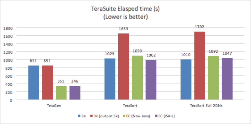
TeraSuite Elapsed Time

Figure 2. TeraGen/ TeraSort Performance

The above results indicate that EC performed more than 50% faster than replication for TeraGen. EC benefited from the parallel writes and the significantly smaller amount of data written. EC writes accounted for 150% of the original data size, compared to 300% for 3x replication, while still providing the same level of fault tolerance.

Two different executions were done for TeraSort tests, the first test with all DataNodes running and the second test where, before the TeraSort test execution, two randomly selected DataNodes were shut down manually. For TeraSort in the failed DataNodes tests, EC performed more than 50% faster when compared to 3x replication, achieving a similar performance to 3x replication with an output file of replication factor 1. Note that, as expected, the TeraSort test with 3x replicated output file performed 40% slower than the default TeraSort with 1x replicated output file, because the 3x replication test writes three times more data than the test with a 1x replicated output file.

The EC performance with two of nine DataNodes shut down was similar to the results with all nine DataNodes running. This similarity is mainly because the end-to-end time measured contains not only the storage time, but also the job execution time. Although two DataNodes were shut down, the NodeManagers were running and the computing power was the same. Therefore, the ‘on-the-fly’ reconstruction overhead is small enough to be insignificant when compared to the computing overhead.

Codec Micro-Benchmark Results

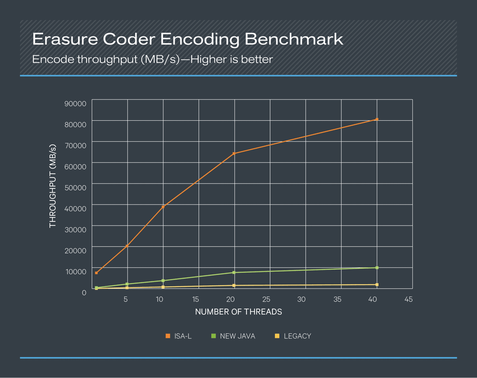
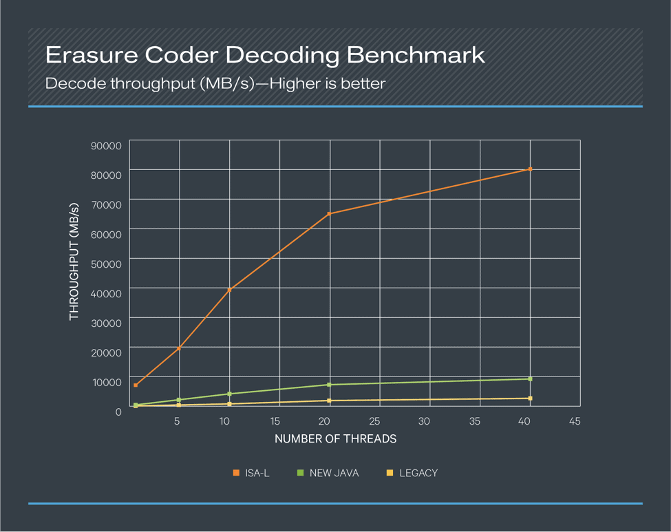
The codec that performs the erasure coding calculations can be an important accelerator of HDFS EC. Encoding and decoding are very CPU-intensive and can be a bottleneck for read/write paths. HDFS EC uses the Reed-Solomon (RS) algorithm, by default the RS (6,3) schema. The following figures show that Intel’s ISA-L coder significantly outperforms both the new Java coder and the legacy coder. These tests were done on the same hardware profile described above with 1 CPU core at 100% utilization.

Erasure Coder Encoding Benchmark

Figure 3. Erasure Coder Encoding Benchmark

Erasure coder decoding benchmark

Figure 4. Erasure Coder Decoding Benchmark

In both the encoding and decoding benchmarks, the ISA-L coder performed about sixteen times better than the new Java coder when single-threaded and performed about eight times better even with 40 concurrent threads. Compared to the legacy coder, the numbers became about 70 times better when single-threaded and about 35 times better with 40 concurrent threads. Based on these results, leveraging the ISA-L coder for HDFS EC offers a great deal of value to any use case. ISA-L is packaged and shipped with CDH 6.1 and enabled by default.

In addition to the benchmarks with different concurrency, some additional tests were done with different buffer sizes. When single threaded, we saw that a buffer size of 64 KB or 128 KB performed about 8% better than a buffer size of 1024 KB. This is likely because the single-threaded test benefitted the most from CPU cache. For five or more concurrent threads, a 1024KB buffer size yielded the best performance. For this reason, the default EC policies of HDFS are all configured to have a cell size of 1024 KB.

DFSIO

A set of DFSIO (Hadoop’s distributed I/O benchmark) tests were run to compare the throughput of 3x replication and EC. In our tests, different numbers of mappers were tested, with each mapper processing a 25GB file. The operating system cache was cleaned before running each test. The result was captured as the overall execution time. Note that the DFSIO tests do not use data locality, so the results can differ slightly from production use cases, where replication can benefit from data locality while EC does not.

DFSIO write elapsed time

Figure 4. DFSIO Write Performance
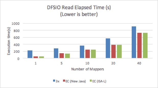
DFSIO read elapsed time

Figure 5. DFSIO Read Performance

EC with ISA-L consistently outperformed 3x replication in both read and write tests.

With only one mapper, EC outperformed 3x replication by 300% on the read test. With an  increased number of mappers, EC was only about 30% faster than 3x replication, because a higher concurrency of mappers creates higher disk I/O contention, which reduces the overall throughput. We also observed that with a single mapper, cross-cluster disk utilization was more than five times higher with EC than with replication; with 40 mappers, disk utilization was at the same level, with EC performing only slightly better.

For the write test, when the number of mappers was low, 3x replication performed better than EC with the new Java codec, but was 30% to 50% slower than EC with ISA-L. With 40 mappers, 3x replication was the slowest, and took more than twice the execution time of EC, because of having to write twice the amount of data (300% vs 150%).

TPC-DS

We conducted comprehensive TPC-DS tests using Hive on Spark to gain insight into the performance for various queries. Tests were run for both ORC and text formats. We ran all the tests three times, and the result below is the average. The complete results are in this spreadsheet for curious readers.

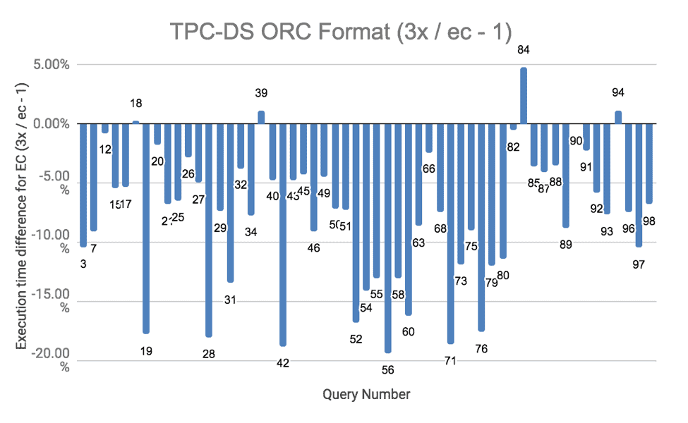
The results of the TPC-DS runs show that EC performed slightly worse than replication in most cases. An important contributing factor in the overall performance drop was the remoteness of  reading and writing erasure-coded data. There were a few CPU intensive queries where EC performed more than 20% slower. The CPU was almost fully used in running these queries. Given that writes are more CPU intensive for erasure-coded data due to parity block computations, the execution time increased. These queries are numbers 28, 31, and 88 for text formats. For a similar reason, the test results were a little worse for erasure coding when ORC file format was used, because data compression used for ORC files increased the overall CPU usage.

TPC-DS ORC format

Figure 6. TPC-DS Performance with ORC format

TPC-DS Text Format

Figure 7. TPC-DS Performance with Text format

Spark

To better understand the performance of EC in end-to-end Spark jobs with different file sizes, several tests were conducted using TeraSort and Word Count on Spark on a different 20-node cluster using the RS(10,4) erasure coding policy. For each test, the overall amount of data was fixed, but different file sizes and numbers of files were configured for testing. We chose to use 600 GB of data for TeraSort and 1.6 TB of data for Word Count. Three series of tests were performed, simulating file sizes that were much smaller than, or similar to, or multiple times larger than the block size (128MB). For the rest of this blog post, we call these three series of tests as small, medium, and large files tests, respectively.

The following table lists the different file sizes used in the tests:

  TeraSort WordCount
  Number of files Size of each input file Number of files Size of each input file Size of each output file
Small files 40,000 15 MB 40,000 40 MB 80-120 bytes
Medium files 4,000 150 MB 4,000 400 MB 80-120 bytes
Big files 1,000 600 MB 1,000 1.6 GB 80-120 bytes

Table 3. Different file sizes used in Spark tests

terasort elapsed time

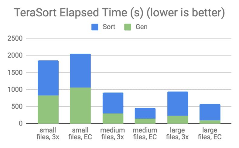
Figure 8. Spark TeraSort Performance for RD(10,4)
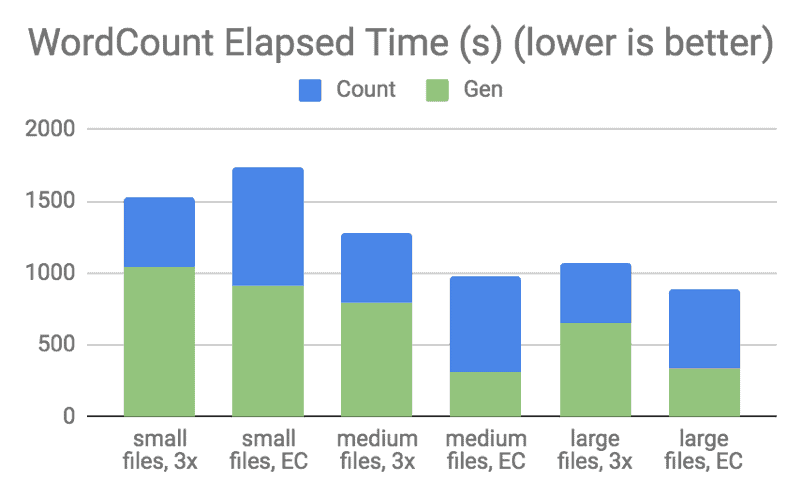
wordcount elapsed time

Figure 9. Spark Word Count Performance for RS(10,4)

In both the graphs, “Gen” means to create the files for the respective job run, which is a write-heavy workload. “Sort” and “Count” mean the execution of the job, including reading the input files from HDFS, executing the tasks, and writing the output files. As stated earlier, the output file size for a Word Count job is typically very small, in the range of several hundred bytes.

From the TeraSort graph above, you can see that EC performed better than 3x replication for medium and large files tests. However, for small file tests, EC performed worse than replication because reading many small blocks concurrently from multiple DataNodes caused a lot of overhead. Note that TeraSort performed slightly worse with large files than with medium files, for both erasure-coded and replicated data, probably because of the increased amount of spilled records in case of large files.

Similar results were seen in the Word Count run. Note that because the Word Count job output files were extremely small, EC consistently performed worse than 3x replication, which is unsurprising considering the increased memory pressure on the NameNode described in the File Size and Block Size section. In addition to that, when the file size is smaller than the EC cell size (1 MB by default), the EC file is forced to fall back to replicating the data into all its parity blocks, yielding effectively four identical replicas with RS(6, 3) and five identical replicas with RS(10, 4). For more information, see the File Size and Block Size section.

Failure Recovery

When one of the EC blocks is corrupted, the HDFS NameNode initiates a process called reconstruction for the DataNodes to reconstruct the problematic EC block. This process is similar to the replication process that the NameNode initiates for files using replication that are under-replicated.

The EC block reconstruction process consists of the following steps:

  1. The failed EC blocks are detected by the NameNode, which then delegates the recovery work to one of the DataNodes.
  2. Based on the policy, the minimum required number of the remaining data and parity blocks are read in parallel, and from those blocks, the new data or parity block is computed. Note that for erasure-coded data, each data block and parity block is on a different DataNode, ideally a different rack as well, making reconstruction a network-heavy operation.
  3. Once the decoding is finished, the recovered blocks are written out to the DataNodes.

One common concern for EC is that reconstruction might consume more resources (CPU, network) in the cluster overall, which can burden performance or cause recovery to be slower when a DataNode is down. Reconstructing erasure-coded data is much more network-intensive than replication, because the data and parity blocks used for the reconstruction are distributed to different DataNodes and usually to different racks. In an ideal setup with sufficient number of racks, each storage block of an erasure-coded logical block is distributed to a different rack; therefore, the reconstruction requires reading the storage blocks from a number of different racks. For example, if RS(6, 3) is used, data needs to be pulled from six different racks in order to reconstruct a block. Reconstruction of erasure-coded data is also much more CPU-intensive than replication because it needs to calculate the new blocks rather than just copying them from another location.

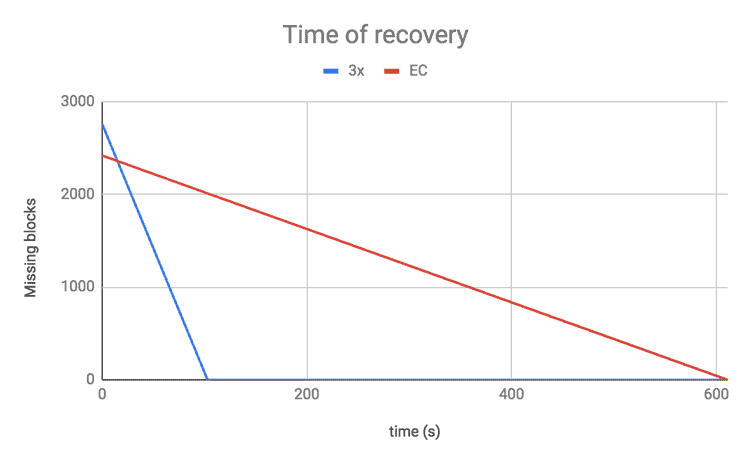
We performed a test in order to observe the impact of reconstruction. We shut down one DataNode on a 20-node cluster and measured the speed of the recovery using the RS(3, 2) erasure coding policy against regular 3x replication. For erasure-coded data, the recovery took six times longer than for 3x replication.

Recovery is usually slower for erasure-coded data than for 3x replication, but if a more fault-tolerant policy is used, it can be less critical. For example when RS(6, 3) is used and if one block is lost, two more missing blocks can still be tolerated. The higher failure tolerance can therefore reduce the priority of reconstruction, allowing it to be done at a slower pace without increasing the risk of data loss. The same is true for losing a rack if there are enough racks so that each data block and parity block is distributed to a different rack. For more information on how erasure-coded data is distributed across racks, see the Locality section of this blog post.

time of recovery

Figure 10. Time of recovery for RS(3,2)

The parameters listed in the Apache HDFS documentation can be tuned to provide fine-grained control of the reconstruction process.

Production Considerations

Besides storage efficiency and single job performance, there are many other considerations when deciding if you want to implement erasure coding for production usage. For information about how to migrate existing data to EC, see the Cloudera documentation.

Locality

From the beginning, data locality has been a very important concept for Hadoop. In traditional HDFS, where data is replicated, the block placement policy of HDFS puts one of the replicas on the node performing the write operation, and the NameNode tries to satisfy a read request from a replica that is closest to the reader. This approach enables the client application to take advantage of data locality and reduces network traffic when possible. DataNodes also have features like short-circuit reads to further optimize for local reads.

For erasure-coded files, all reads and writes are guaranteed to have remote network traffic. In fact, the blocks are usually not only read from remote hosts but also from multiple different racks.

By default, EC uses a different block placement policy from replication. It uses a rack-fault-tolerant block placement policy, meaning that the data is distributed evenly across the racks. An erasure-coded block is distributed to a number of different DataNodes equal to the data-stripe width. The data-stripe width is the sum of the number of data blocks and parity blocks defined by the erasure coding policy. If there are more racks than the data-stripe width, then an erasure-coded block is stored on a number of randomly chosen racks equal to the data-stripe width, that is, each of the DataNodes is selected from a different rack. If the number of racks is less than the data-stripe width, then each rack is assigned a number of storage blocks that is a little more than the value of data-stripe width/number of racks. The rest of the storage blocks are distributed to other DataNodes that hold no other storage blocks for the logical block. For more information, checkout Cloudera’s documentation about Best Practices for Rack and Node Setup for EC.

For this reason, EC performs best in an environment where rack-to-rack bandwidth is not oversubscribed or has very low oversubscription. Network throughput should be carefully monitored when increasing the overall mix of EC files. This effect is also one of the biggest reasons why Cloudera recommends to start using EC with cold data. For more information, see Cloudera’s documentation.

File Size and Block Size

Other important considerations for EC are file size and block size. By default, the HDFS block size in CDH is 128 MB. With replication, files are partitioned into 128MB chunks (blocks) and replicated to different DataNodes. Each 128MB block, though, is complete within itself and can be read and used directly.  With EC, each of the underlying data blocks and parity blocks is located in a different 128MB regular block. Reading data from a block means reading data from all blocks in the block group.  A block group is (128 MB * (Number of data blocks)) in size. For example, RS(6, 3) will have a block group of 768 MB (128 MB * 6).

It is important to consider the implications of that model on the memory usage of the NameNode, specifically the number of blocks in the NameNode block map. For EC, the bytes/blocks ratio is worse for small files which increases the memory usage of the NameNode. For RS(6,3) the NameNode stores the same amount of block objects, nine block objects, for a 10MB file as for a 768 MB file. Comparing it with 3x replication, a 10MB file with 3x replication means three block objects in the NameNode; a 10MB file with EC (RS(6, 3)) means nine block objects in the NameNode!

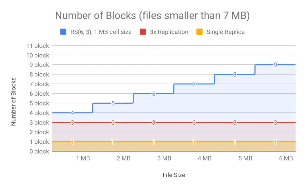
For very small files of sizes smaller than the value of data blocks * cell size (in case of RS(6, 3) it is 6 * 1MB), the bytes/blocks ratio is also bad. This is because the number of actual data blocks is less than the data blocks defined by the erasure coding policy, though the number of parity blocks is always the same. For example, in the case of RS(6,3) with a cell size of 1 MB, a 1MB file consists of one data block, rather than six, but it still has three parity blocks. A 1MB file would therefore require four block objects in total. If 3x replication were used, the same file would require only three block objects. You can see the number of blocks for different file sizes in Figure 11 and Figure 12.

number of blocks (files smaller than 7mb)

Figure 11. Number of Blocks in NameNode for Different File Sizes (files larger than 7MB)
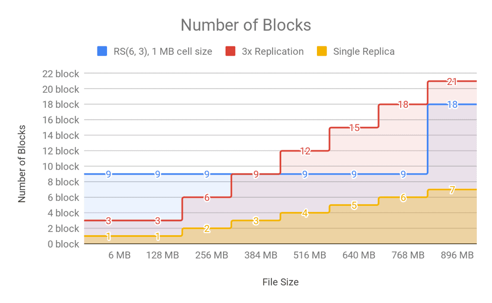
number of blocks

Figure 12. Number of Blocks in NameNode for Different Files Sizes

As shown in the above figures, the number of blocks is linear to file size for replication, but is a step function for EC because of the nature of the striping layout. For this reason, EC may aggravate memory pressure on the NameNode in clusters with a high number of small files. (For more information on the small files problem, see this blog post). Large files are better suited to EC, because the block count for the final partial block group is amortized over the whole size of the file. An ideal workflow would include a process to merge and compact the small files into a large file and apply EC to that compacted large file. For more information, see this documentation about compacting small files using Hive.

Decoding and Recovery

When reading an erasure-coded file in HDFS, reading from the data blocks and constructing the logical block (file content) does not have to pay any EC encoding or decoding cost. However, if any of the data blocks cannot be read—for example because the DataNode holding it is down, or the block is corrupt and being reconstructed—HDFS will read from the parity blocks and decode into a logical block. Although the problematic data block is reconstructed later in an asynchronous fashion, the decoding consumes some CPU. From Figure 4, this decoding adds very minor overhead to the overall performance.

Conclusion

Erasure coding can greatly reduce the storage space overhead of HDFS, and, when used correctly for files of appropriate sizes, can better utilize high-speed networks for a higher throughput. In the best case scenario, on a network with completely sufficient bandwidth, with the Intel ISA-L library and Hadoop ISA-L coder, read and write performances are expected to be better than the traditional 3x replication for large files. Cloudera has integrated erasure coding into CDH with first-class enterprise support. However, it is strongly recommended that customers evaluate their current HDFS usage and plan to on-board files to EC accordingly. When doing so, keep in mind that the small files problem is exacerbated when EC is used for small files.

For a step-by-step guide on how to set up HDFS erasure coding in CDH, see Cloudera’s documentation. For best practices for using erasure coding with Hive, see this documentation.

Xiao Chen is a member of the Apache Hadoop PMC.
Sammi Chen is a member of the Apache Hadoop PMC.
Kitti Nanasi is a Software Engineer at Cloudera.
Jian Zhang is a Software Engineer at Intel.

The post HDFS Erasure Coding in Production appeared first on Cloudera Engineering Blog.

Apache Phoenix for CDH

$
0
0

Apache Phoenix for CDH: Best New Feature for DBMS

Cloudera is adopting and will be supporting Apache Phoenix for CDH while it integrates it for its Cloudera Data Platform on a go-forward basis.

Cloudera’s CDH releases have included Apache HBase which provides a resilient, NoSQL DBMS for customers operational applications that want to leverage the power of big-data.  These applications have grown into mission important and mission critical applications that drive top-line revenue and bottom-line profitability.  These applications include customer facing applications, ecommerce platforms, risk & fraud detection used behind the scenes at banks or serving AI/ML models for applications and enabling further reinforcement training of the same based on actual outcomes.

However, for many customers, HBase has been too daunting a journey — requiring them to learn 

  • A new data model as HBase is a wide-table schema supporting millions of columns but no joins and 
  • Using Java APIs instead of ANSI SQL 

They have asked to be able to use more traditional schema design that resembles that provided by Oracle or MySQL and been willing to make some trade-offs on flexibility e.g., 

  • They are willing to use provided data types instead of defining their own
  • They are willing to give up the flexibility to have a single column have multiple types depending on the row in exchange for a single type in a single row

To enable customers to have an easy on-ramp to the other benefits of Apache HBase (unlimited scale-out, millions of rows, schema evolution, etc) while providing RDBMS-like capabilities (ANSI SQL, simple joins, data types out of the box, etc), we are introducing support for Apache Phoenix on CDH.

Apache Phoenix on CDH

For everyone else, Phoenix based applications also benefit from behind-the-scenes HBase optimizations, making it easier to get better HBase performance.  For example, Phoenix implements salting of primary keys — so HBase users don’t have to think through this aspect of key design.

Further, Phoenix based applications can co-exist with HBase applications — meaning you can use a single HBase cluster to support both.  With Phoenix, customers can continue to use their favorite BI & dashboarding tools just like they did with Hive & Impala in the past.  When using Phoenix, they can also choose to directly use Phoenix with those tools in addition to the option of using Hive / Impala eliminating a step for new implementations.Cloudera SDX with NiFi Spark Phoenix Hbase Hue Hive

From a security and governance perspective (SDX), in CDH, Phoenix uses HBase ACLs for role based access control for Phoenix tables.  Phoenix also uses HBase integration into Cloudera Navigator for audit information.

Initially, Cloudera will make a Phoenix 4.14.1 parcel available to CDH 5.16.2 customers.  Soon there-after, we will make a Phoenix 5.0 parcel available to CDH 6.2 customers.

Existing HDP customers already have Apache Phoenix support and almost half of HBase users using HDP currently use Phoenix as well speaking to its popularity in the HBase user community.

Download Apache Phoenix for CDH 

Build mission-critical applications using Apache Phoenix. Download the software here.


Frequently asked questions about Phoenix


Q) What are the workloads that Phoenix should be used for

Phoenix supports the same use cases as HBase, primarily low-latency, high concurrency workloads.  However, Phoenix makes it simpler to also leverage the underlying data for dashboarding & BI purposes

Q) What is the authorization mechanism with Phoenix?

Phoenix depends on HBase for authorization.  For CDH customers, this utilizes HBase ACLs. For HDP customers, this is through HBase-Ranger integration

Q)  What’s the scalability of Phoenix? What’s the largest known cluster?

Phoenix scales to hundreds of TB of data.  The largest customer has over 0.5 PB of data that is managed by Phoenix.  Specifics on use cases can be found in the PhoenixCon archives and in the archives for NoSQL day videos earlier this year in users own words & slides.

Q) Does Phoenix support geo spatial secondary indexing? What level of support spatial data?

It has limited support for geo-spatial data.  However, GeoMesa provides a geospatial layer on HBase that can support this need and integrated with customer applications.  Phoenix, GeoMesa as well as JanusGraph and OpenTSDB can all co-exist in a single HBase cluster.  

Q) How do you create and use an Index?

See Phoenix Secondary Indexing page for details on indexing.  From Phoenix 4.8.0 onward, no configuration changes are required to use local indexing. 

Q)  Is there a limit on number of columns you can put on index?

Like in an RDBMS, an index is essentially a separate table with the index and a link to the source data. If you index all columns you defeat the purpose by maintaining two identical tables.  Indexes should be used judiciously as there is some non-trivial overhead on write (global indexes) or read (local indexes).

The post Apache Phoenix for CDH appeared first on Cloudera Engineering Blog.

Viewing all 426 articles
Browse latest View live